Raising the Curtain: Getting Started with overtureR • overtureR

# install if needed:
install.packages("overtureR")

library(overtureR)
library(ggplot2)
library(dplyr)
library(sf)

This vignette demonstrates how to use overtureR to access and visualize Overture Maps data, focusing on a practical example in Washington, DC: finding the theater.

Overture Maps is an open-source mapping initiative aimed at developers who build map services or use geospatial data. It provides a collaborative, globally-referenced, and quality-assured dataset with a structured schema. This makes it an excellent resource for creating reliable and interoperable map products. Using overtureR, we can easily tap into this rich dataset. In this guide, we’ll walk through the process of:

Fetching the boundary of Washington, DC
Locating Ronald Reagan National Airport
Finding the Kennedy Center theater
Getting to the Kennedy Center with public transit

open_curtain() function is our primary tool for accessing Overture Maps data. We’ll start by using open_curtain() to retrieve the DC boundary and pinpoint the airport:

# Washington, DC boundary
dc <- open_curtain("division_area") |>
  filter(subtype == "region", region == "US-DC") |>
  collect()

# adding a bounding box makes the query faster:
dc_catchment <- st_geometry(dc) |>
  # 10 miles from DC
  st_buffer(10 * 1609.34) |>
  st_bbox()

reagan_airport <- open_curtain("place", spatial_filter = dc_catchment) |>
  filter(
    names$primary == "Ronald Reagan Washington National Airport",
    categories$primary == "airport"
  ) |>
  collect()
#> OGR: Unsupported geometry type

print(reagan_airport)
#> Simple feature collection with 1 feature and 15 fields
#> Geometry type: POINT
#> Dimension:     XY
#> Bounding box:  xmin: -77.04384 ymin: 38.84906 xmax: -77.04384 ymax: 38.84906
#> Geodetic CRS:  WGS 84
#> # A tibble: 1 × 16
#>   id                       geometry bbox$xmin version sources      names$primary
#> * <chr>                 <POINT [°]>     <dbl>   <int> <list>       <chr>        
#> 1 08f2aa87b1c… (-77.04384 38.84906)     -77.0       0 <df [1 × 5]> Ronald Reaga…
#> # ℹ 15 more variables: bbox$xmax <dbl>, $ymin <dbl>, $ymax <dbl>,
#> #   names$common <list>, $rules <list>, categories <df[,2]>, confidence <dbl>,
#> #   websites <list>, socials <list>, emails <list>, phones <list>,
#> #   brand <df[,2]>, addresses <list>, theme <chr>, type <chr>

By default, open_curtain would search through every “place” (aka point of interest) in the world - an enormous dataset. Obviously, that’s too much to load into most computers’ memory, so open_curtain does this lazily. Only after calling collect_sf does it load data onto your computer. So we filter the data first, spatially and by name, like so:

fetch the boundary of Washington, DC from the “division_area” dataset;
filter for the specific region we wanted;
create a spatial buffer around DC to define our area of interest for subsequent queries; and
locate Ronald Reagan National Airport using the “place” dataset, filtering by name and category.

Afterwards, collect_sf brings the only the data need into memory. For more on lazy programming, see the dbplyr documentation.

Now that we’ve set the stage with our starting point, let’s spotlight our destination. In the next code block, we’ll locate the Kennedy Center:

reagan_plot <- ggplot() +
  geom_sf(data = dc, fill = "purple", alpha = 0.05) +
  geom_sf(data = reagan_airport, color = "red", size = 4) +
  geom_sf_label(
    data = reagan_airport, nudge_y = 0.01, aes(label = names$primary)
  ) +
  theme_minimal() +
  theme(
    axis.title = element_blank(),
    axis.text = element_blank(),
    axis.ticks = element_blank(),
    panel.grid = element_blank()
  )

reagan_plot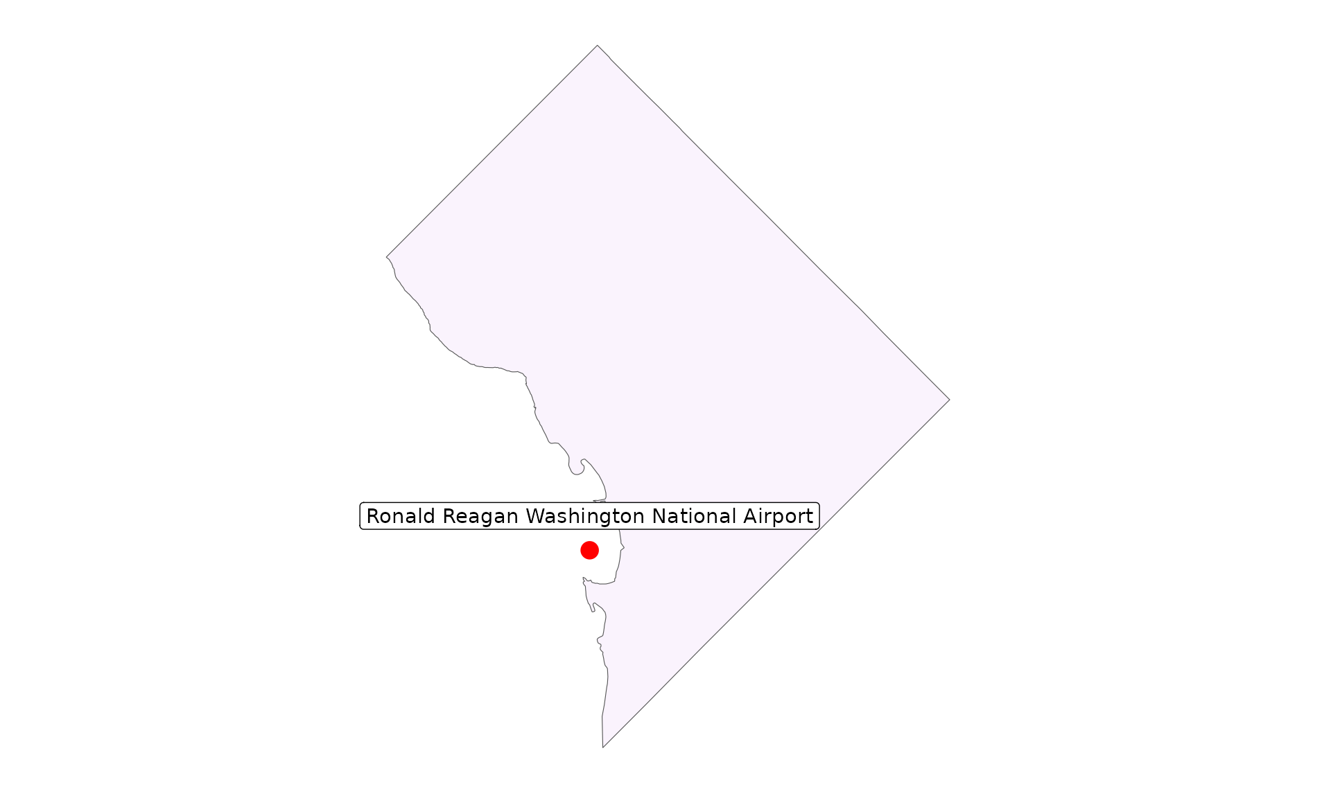

In this code, we’ve queried the “building” dataset within our defined DC area. We used a text filter to find buildings with “The Kennedy Center” in their name. This demonstrates overtureR’s ability to perform text-based searches within the Overture Maps dataset.

To get to the theater, we’ll need to know our transit options. The following code showcases overtureR’s capacity to handle more complex spatial and attribute queries:


kennedy_center <- open_curtain("building", st_bbox(dc)) |>
  filter(grepl("Kennedy Center", names$primary)) |>
  collect()


kennedy_plot <- reagan_plot +
  geom_sf(data = kennedy_center, fill = "green") +
  geom_sf_label(data = kennedy_center, nudge_y = 0.01, aes(label = names$primary))
kennedy_plot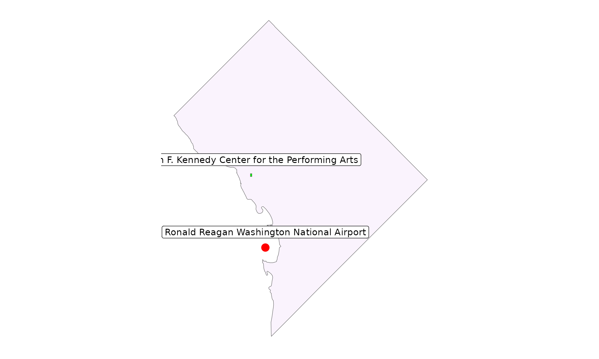

In the code above, we’ve created a bounding box that encompasses both the airport and the Kennedy Center, plus a one-mile buffer. We then used this to filter the “segment” dataset for rail transit, specifically the Blue Line of the DC Metro.

For the grand finale, we’ll create a map that displays all the elements we’ve gathered:

# filter town to areas that are within ~1 mile of our two points
kennedy_reagan_bbox <- bind_rows(kennedy_center, reagan_airport) |>
  st_bbox() |>
  st_as_sfc() |>
  st_buffer(1 * 1609.34) |>
  st_bbox()

dc_transit <- open_curtain("segment", kennedy_reagan_bbox) |>
  filter(
    subtype == "rail",
    # filter to the Blue Line of the DC Metro
    grepl("Metro", names$primary),
    grepl("Blue", names$primary)
  ) |>
  select(id, names, geometry) |>
  collect()

print(dc_transit)
#> Simple feature collection with 22 features and 2 fields
#> Geometry type: LINESTRING
#> Dimension:     XY
#> Bounding box:  xmin: -77.07099 ymin: 38.81561 xmax: -76.96203 ymax: 38.90138
#> Geodetic CRS:  WGS 84
#> # A tibble: 22 × 3
#>    id                               names$primary                       geometry
#>  * <chr>                            <chr>                       <LINESTRING [°]>
#>  1 0852aa87bfffffff043d7d4cb96bc842 Washington Metro … (-77.04351 38.8519, -77.…
#>  2 0852aa87bfffffff043f7d4fefed55e2 Washington Metro … (-77.05255 38.81561, -77…
#>  3 0892aa87b0c7ffff043f5f8927117f84 Washington Metro … (-77.05915 38.86413, -77…
#>  4 0892aa87b0c7ffff043f5f87f060d849 Washington Metro … (-77.05907 38.86444, -77…
#>  5 0862aa87b7ffffff047d7dd09f3c4f01 Washington Metro … (-77.0448 38.85507, -77.…
#>  6 0862aa87b7ffffff047f7fd8ec04aa8b Washington Metro … (-77.0433 38.85196, -77.…
#>  7 0872aa87b0ffffff043dff5fd720ea58 Washington Metro … (-77.05918 38.86414, -77…
#>  8 0872aa87b0ffffff043fff6322f465a8 Washington Metro … (-77.04461 38.85512, -77…
#>  9 0862aa87b7ffffff043ddbfe124c8a34 Washington Metro … (-77.05269 38.87024, -77…
#> 10 0862aa87b7ffffff043f5d0044cff8a1 Washington Metro … (-77.05904 38.86444, -77…
#> # ℹ 12 more rows
#> # ℹ 2 more variables: names$common <list>, $rules <list>

This final step uses ggplot2 to create a map that displays the airport, the Kennedy Center, and the Metro Blue Line connecting them. This visualizes the route from our arrival point to our theatrical destination.

kennedy_plot +
  geom_sf(data = dc_transit, color = "blue") +
  coord_sf(
    xlim = c(kennedy_reagan_bbox[["xmin"]], kennedy_reagan_bbox[["xmax"]]),
    ylim = c(kennedy_reagan_bbox[["ymin"]], kennedy_reagan_bbox[["ymax"]]),
  )

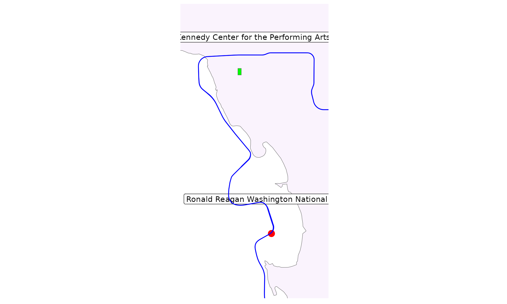
Perfect, it looks like we can take the blue line straight there. Break a leg!